Tutorial
This chapter describes step-by-step how to use the Cubes. You will learn:
- model preparation
- measure aggregation
- drill-down through dimensions
- how to slice&dice the dube
The tutorial contains examples for both: standard tool use and Python use. You don’t need to know Python to follow this tutorial.
Data Preparation
The example data used are IBRD Balance Sheet taken from The World Bank. Backend used for the examples is sql.browser.
Create a tutorial directory and download IBRD_Balance_Sheet__FY2010.csv.
Start with imports:
>>> from sqlalchemy import create_engine
>>> from cubes.tutorial.sql import create_table_from_csv
Note
Cubes comes with tutorial helper methods in cubes.tutorial. It is advised not to use them in production; they are provided just to simplify the tutorial.
Prepare the data using the tutorial helpers. This will create a table and populate it with contents of the CSV file:
>>> engine = create_engine('sqlite:///data.sqlite')
... create_table_from_csv(engine,
...                       "IBRD_Balance_Sheet__FY2010.csv",
...                       table_name="ibrd_balance",
...                       fields=[
...                             ("category", "string"),
...                             ("category_label", "string"),
...                             ("subcategory", "string"),
...                             ("subcategory_label", "string"),
...                             ("line_item", "string"),
...                             ("year", "integer"),
...                             ("amount", "integer")],
...                       create_id=True
...                   )
Analytical Workspace
Everything in Cubes happens in an analytical workspace. It contains cubes, maintains connections to the data stores (with cube data), provides connection to external cubes and more.
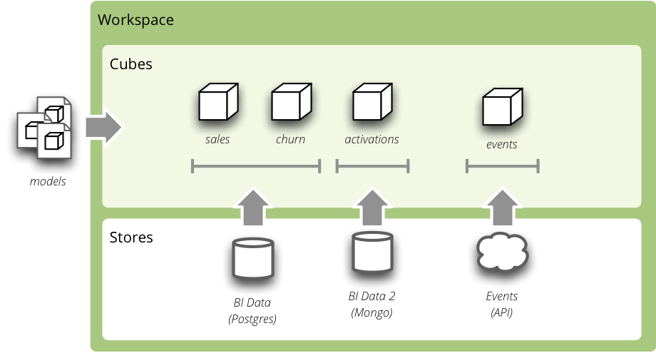
Analytical workspace and it’s content
The workspace properties are specified in a configuration file slicer.ini (default name). First thing we have to do is to specify a data store – the database containing the cube’s data:
[store]
type: sql
url: sqlite:///data.sqlite
In Python, a workspace can be configured using the ini configuration:
from cubes import Workspace

workspace = Workspace(config="slicer.ini")
or programatically:
workspace = Workspace()
workspace.register_default_store("sql", url="sqlite:///data.sqlite")
Model
Download the tutorial model and save it as tutorial_model.json.
In the slicer.ini file specify the model:
[workspace]
model: tutorial_model.json
For more information about how to add more models to the workspace see the configuration documentation.
Equivalent in Python is:
>>> workspace.import_model("tutorial_model.json")
You might call import_model() with as many models as you need. Only limitation is that the public cubes and public dimensions should have unique names.
Aggregations
Browser is an object that does the actual aggregations and other data queries for a cube. To obtain one:
>>> browser = workspace.browser("ibrd_balance")
Compute the aggregate. Measure fields of AggregationResult have aggregation suffix. Also a total record count within the cell is included as record_count.
>>> result = browser.aggregate()
>>> result.summary["record_count"]
62
>>> result.summary["amount_sum"]
1116860
Now try some drill-down by year dimension:
>>> result = browser.aggregate(drilldown=["year"])
>>> for record in result:
...     print record
{u'record_count': 31, u'amount_sum': 550840, u'year': 2009}
{u'record_count': 31, u'amount_sum': 566020, u'year': 2010}
Drill-down by item category:
>>> result = browser.aggregate(drilldown=["item"])
>>> for record in result:
...     print record
{u'item.category': u'a', u'item.category_label': u'Assets', u'record_count': 32, u'amount_sum': 558430}
{u'item.category': u'e', u'item.category_label': u'Equity', u'record_count': 8, u'amount_sum': 77592}
{u'item.category': u'l', u'item.category_label': u'Liabilities', u'record_count': 22, u'amount_sum': 480838}